Tutorials |||| Installing and Using ns-2 | Installing Rapid in ns-2 | Using Tmix in ns-2

A Short Tutorial for Installing and Using ns-2 to Simulate Rapid TCP

This guide is dedicated (but not limited in its utility) to UNC-CH people who are interested in using ns-2 to simulate and test Rapid packet-scale congestion control. This page should give you enough information to get started with using ns-2 to test Rapid. For general tutorials of ns-2, see the ns-2 website.

1. Install ns-2
2. Add Rapid to ns-2
3. Download my Example Experiment
4. Run an ns-2 Experiment
5. Process Experiment Output
6. Visualize Data with Gnuplot

Step 1: Install ns-2

1. Log on to the Rapid machine, and cd into wherever you want to install ns. (I extracted the installation file into my playpen directory.)
2. Download and install ns-2.35:
   % cd /playpen/lovewell/
   % wget http://www.isi.edu/nsnam/dist/release/RC8/ns-allinone-2.35-RC8.tar.gz
   % tar xzf ns-allinone-2.35-RC8.tar.gz
   % cd ns-allinone-2.35-RC8/
   % ./install
   
   I used RC8, but since then more candidates have been released. You can check for other versions here. These instructions assume RC8.
3. Follow any instructions given at the end of the installation output. (You probably need to add some things to your environment variables. I did this by editing .cshrc in my home directory.)
4. Make sure that the ns-allinone-2.35-RC8/bin directory is in your path variable. (I did this by editing .cshrc in my home directory.)
5. You may need to restart your shell for the variable changes to take effect. Verify that you're using the right version of ns with the command which ns.

Step 2: Add Rapid to ns-2

Follow these instructions to add Rapid to your ns-2 installation. Although the instructions cite v2.34, all things should be parallel in v2.35. As far as I know, the patch should still work (but I haven't tested it). You should use v2.35 because it has the appropriate version of Tmix built in.

Internally, copies of tcp-rapid.cc, tcp-rapid.h, rapid-sink.cc, and rapid-sink.h are available in the /playpen/lovewell/ns/rapid/ directory on the rapid.cs.unc.edu machine.

Note: I had to install ns, and then make the changes necessary to install Rapid. I got lots of errors if I tried to add the Rapid code before actually installing ns.

Step 3: Download my Example Experiment

I created files to run a simple experiment. Download and extract this folder wherever you please. All commands should be run from the example/ directory.

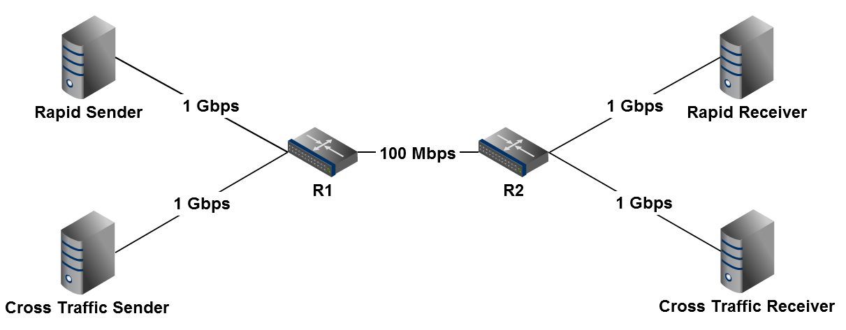
The example files simulate a network very similar to the one we used in the "Impact of Cross Traffic Burstiness on the Packet-scale Paradigm" paper. A Rapid sender and a cross traffic sender share a single, bottleneck link. The cross-traffic sender is bursty, with an on period of T_on, and an off period of T_off between each burst. While on, the cross traffic sender sends at a constant rate of R_on.

Step 4: Run an ns Experiment

The TCL code to run the ns simulation of the above network is located in example/source.tcl.

To simulate a sender in ns, three things are required. First, you must create a node. Next, you must a TCP (such as Rapid or NewReno) or UDP source that will handle sending out data according to the specified protocol, and attach it to the node. Then, you must create a data application and attach it to the TCP/UDP source.

To simulate a receiver in ns, you must attach a sink to a node.

To run the source file, use the command ns source.tcl from the example/ directory. For more information about how to use TCL, see the ns by Example tutorial.

Some tips:

• Comments are created using a "#" sign. If you want to put a comment on the same line as some code, use a semicolon after the code (for example, set capacity "100Mbps"; # bottleneck link speed). You can also use a semicolon to put multiple commands on one line.
• I use the link delay to create a specified RTT.
• The run time of your experiment is directly correlated with how much data you record. Thus, it is important to record as little as possible to get the data you need!
• It seems that trace-all must be used before any router declarations. (I don't know why.) Use this option very sparingly or for small experiments because it records much more data than you'll need.
• trace-queue must be used after the routers for the link it is tracing have been declared. You'll probably be able to get by with just using trace-queue on the bottleneck link.
• To save space, you can pipe output through gzip. You'll have to unzip the data (temporarily) for processing.

Step 5: Process Experiment Output

Now that you've run an experiment and generated some data, you can process the data to model interesting things. A queue processing script and a throughput/utilization processing script are located in the example/process/ directory.

Check out this super-useful guide for more information about the structure of the output trace.

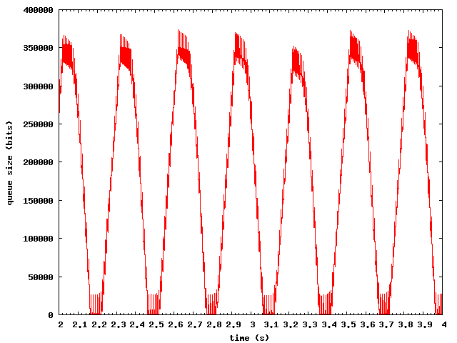
To get data for the queue size at the bottleneck router, run this command from the example/ directory:

where process/queue_size.py is the queue processing script and data/out.gz is the location of the output file containing (gzipped) trace data for the bottleneck link (output by the ns experiment file). The portion < gunzip -c data/out.gz unzips the trace data to stdout and redirects the result to stdin for the processing script. The portion > data/queue.txt redirects the output of the processing script to a file.

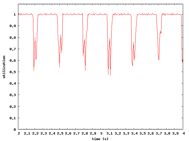
To get utilization data for the bottleneck link, run the command:

where process/throughput.py is the location of the throughput processing script, 100000000 is the capacity, in bits, of the bottleneck link and 0.008 is the granularity, in seconds, at which you want to aggregate the utilization data.

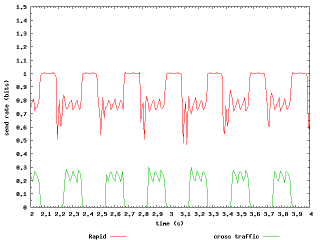
To get send rate data for Rapid traffic, use only the portion of the trace data that refers to traffic going from the Rapid sender (router 2) to the Rapid receiver (router 3):

Similarly, to get send rate data for cross traffic, use only the portion of the trace data that refers to traffic going from the cross traffic sender (router 4) to the cross traffic receiver (router 5):

Some tips:

• Each router is identified in the output using an integer, starting from 0. The identifiers are assigned by ns in the order that the routers are declared.
• If your data appears too erratic, try a larger granularity (for example, aggregate data every 5 ms instead of every 1 ms).

Step 6: Visualize Data with Gnuplot

I used Gnuplot to visualize the processed data. Sample gnuplot scripts are located in the example/plot/ directory.

To use a gnuplot script, use the command:

Output plots for the example experiment, using the data as gathered above:

• Rapid and cross traffic sending rates
• Bottleneck router queue size
• Bottleneck link utilization

Some tips:

• Put output where you can see it easily. I like to output to somewhere in my public_html/ directory.