Physically-Based Modeling
Homework 2
Basic Application
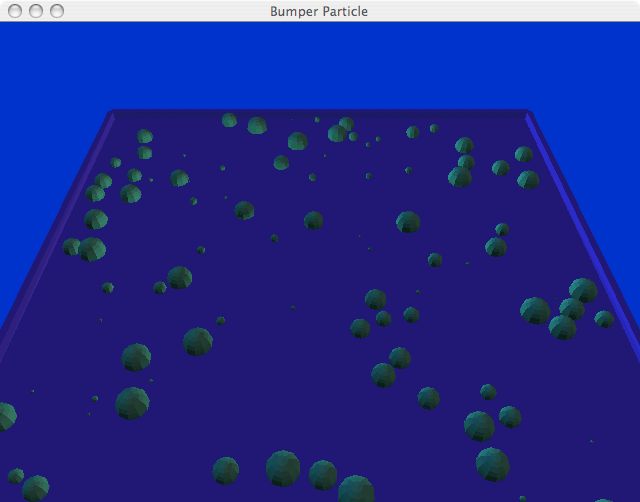 |
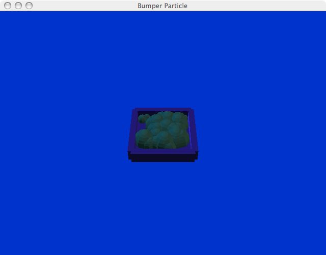
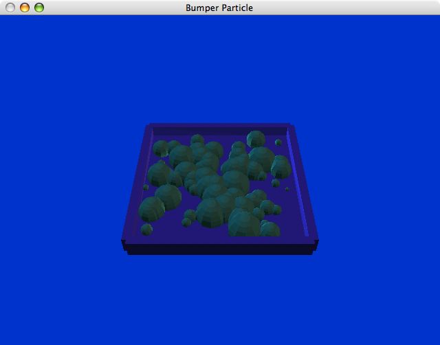
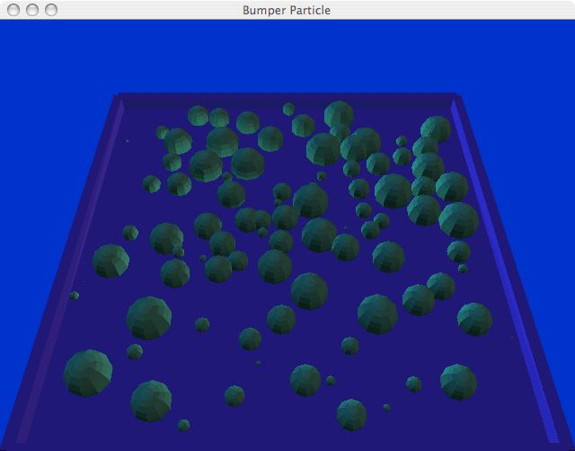
The general set up for assignment 2. There are n objects in a bounded table, moving around in R^2. In the experiments, when the object radii are non-uniform, the radii are generated by the function(srand() * 2), where srand generates a random real number between 0 and 1. |
A screenshot of Homework 2 |
|
Problem A
PQP is used as the collision detection library and timing results are conducted on an Apple iBook G4 1.2 GHz PPC with 1.25 GB ram and OS X 10.4.10. Times reported represent the average time to check and handle collisions where the averages are calculated from 50 samples and times are collected using the unix sys/times library. When checking for inter-object collisions, the implementation for Problem A uses a "brute force" approach, where every object is checked against all other objects for a collision.
To handle collisions and avoid penetrating objects, we maintain the clear set, a set of collisions which have recently collided and are waiting to separate. If the pair, p, is in collision, we check if p is in the clear set, if it is we do nothing. If it is not we handle the collision by reversing the velocity vectors of both objects and add p to the the clear set. If p is not in collision and p is in the clear set, we remove p from the clear set.
Problem B
Experement 1
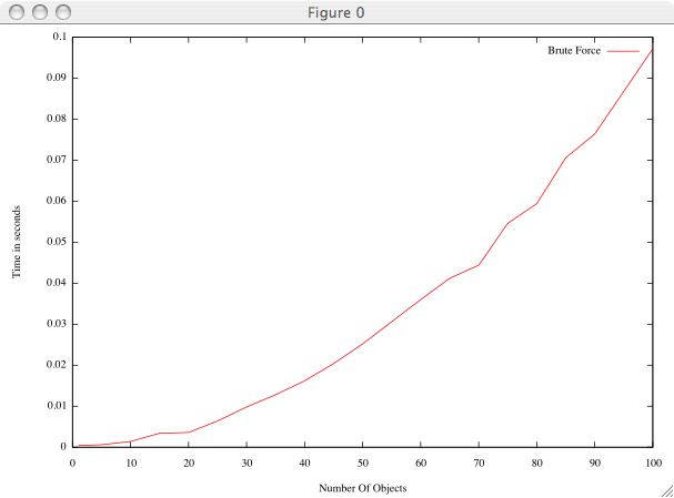 |
For the first experiment we studied the result of increasing the number of objects which are being tested for collision. We tested from 1 to 100 objects in 5 object increments and recorded the results. This graph increases polynomially, which would be expected since we are doing n^2 object based collision checks. |
Experement 2
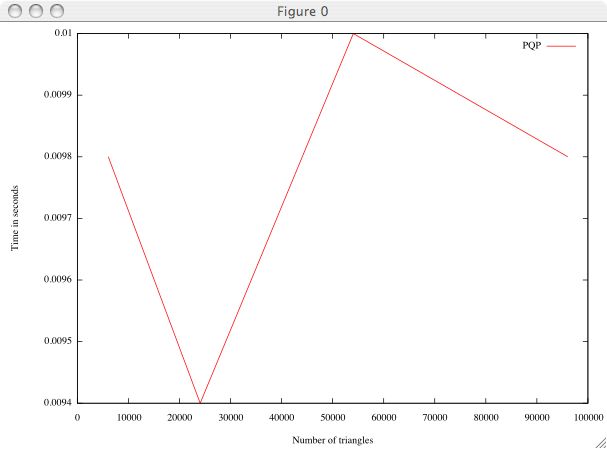
For the second experiment we investigated changing the complexity of the models. This was achieved by refining the increment along phi and theta for our sphere primitive, "roundness". The values ranged from 10 - 40 in 10 unit increments. Testing was done with 30 objects. The graph below shows the time for checking and handling collisions as a function of the number of triangles. Experimentally, it appears that the complexity does not significantly effect the performance of the collision detection. This is because even though the model is more complex, the hierarchy still allows for separations to be found at a high level. |
 |
Experement 3
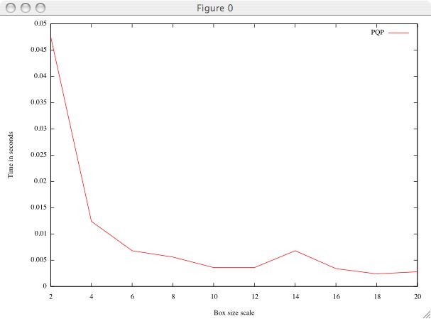 |
For the third experiment we saw how the algorithm responds to relative size of the objects with respect to the bounding space. This was achieved by growing and shrinking the bounding space while maintaining the same number of objects at the same size. Below shows examples where the size of the bounding space is 5, 10, and 20. Experiments were carried out by testing sizes between 2 and 20 in increments of size 2. When the objects are very large with respect to the space the time to check collisions is larger, but very quickly decreases . This is most likely caused by the objects being close together, causing more of the hierarchy to be traversed before a separation can be found if there is no collision. Also in these cases there are more collisions, which also causes the hierarchy to be further traversed. |
Problem C
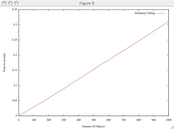
Delaunay Culling
Since we are now making the assumption that all objects are spheres of the same size we can begin by considering the generalization of the Voronoi diagram which is known as the Voronoi diagram of additively weighted points, or the AW-Voronoi for short. Informally , in R^2 AW-Voronoi is the Voronoi diagram of a set of disks, or weighted points, s_i= (p_i, w_i) such that p_i \in R^2, w_i \in R and the distance from a point x to s_i is defined as \delta(x, s_i) = | x - p_i | - w_i. It can be show that AW-Voronoi is unaffected by additively scaling the weights of all points. This fact can then be used to show that if all the weights are the same, computing the AW-Voronoi diagram can be reduced to computing the Voronoi diagram of a set of points. (see David Millman, Degeneracy Proof Predicates for the Additively Weighted Voronoi Diagram for more formal treatment of this topic and further references).
Since our problem can be simplified to finding collisions between circles we could calculate the dual of AW-Voronoi, the Apollonius graph, iterate over all the edges, and each edge would give us the pairs which need to be tested for collisions. As all of our objects are the same size, we could use the facts from above and simple calculate the Delaunay Triangulation, iterate over the edges of the triangulation checking for collisions. Hence the name Delaunay Culling.
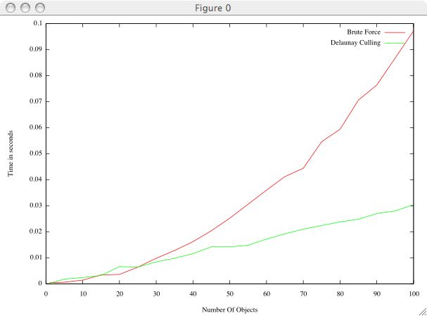
For the assignment, this was implemented and tested with CGAL. Experimentally this method is substantially faster then the "brute force" approach of part a. Below shows a comparison of experiment A from part 1 run with Delaunay Culling and "Brute Force". Also shown is the result of using Delaunay Culling to test up to 1000 objects in incraments of 50.